


Electronics
Lab Power Supplies: 5 Things To Consider When You Invest In Them

The lab power supplies are used so that they can act as a voltage regulation or current regulation power supply. The range of voltage regulation is from 0V to 30V and the range of current is from 0A to 5A. The output by these power supplies are set by the rotary switches with the value displayed on a LCD display. These lab power supply products have low ripple and noise and high reliability as well as high accuracy.
To choose the best or most appropriate lab power supply for a particular application, one must determine the answers to certain important questions and understand the basics of how power supplies are specified. So while looking for a lab or bench power supply, a person must consider some of the important points in order to save substantial time as well as money in the system configuration process.
Things to consider while investing on lab power supplies:
1.Power, voltage and current requirements for the devices which are under test
The power envelopes vary from one power supply to another. In the rectangular power envelope type of supply, any load current is supplied which does not depend on the voltage level.
Another variety has multiple rectangular envelopes for various ranges of voltages and that also offers the option of higher values of one perimeter at the expense of another perimeter.
Then there are those which are capable of delivering hyperbolic envelopes that provide even more continuous transition than multi-range power supplies, in this kind of power supply, one parameter is inversely proportional to the other parameter. The high-power output supplies tend to have either a multi-range or a hyperbolic envelope.
2. Parameters
Accuracy: The accuracy provides the information regarding the closeness between the regulated parameter and its theoretical value. The uncertainty in output is mostly because of error terms in case of digital-to-analogue converter (DAC). The accuracy of the setting is tested by measuring the regulated variable with a traceable, precision measurement supply that can be connected to the output of the power supply.
Resolution: The smallest change in voltage or current setting that can be selected on power supply is known as resolution. The different specifications of resolution, can limit the number of discrete levels that can settle, a DAC which has more bits can produce finer resolution.
But the resolution can be less than the number of bits in the DAC if there is any requirement of correction for offset and gain errors. Setting resolution is either expressed as an absolute unit value or a percentage of full value.
Accuracy of readback: This provides the information regarding how accurate the internally-measured values are compared to the theoretical value of the output voltage.
Stability: The performance of the power supply will change inevitably as it ages. So you must choose a lab power supply which can work properly for a longer time period and for maintaining long term stability regular verification and calibration is required.
Temperature stability: There is a specific temperature range between which the accuracy of power supply is specified. The temperature generally ranges between 20 degree C and 30 degree C.
3. Required output accuracy level: It is important for an individual to review the power supply’s output accuracy and readback specifications for the accurate control of the voltage at the load for experimentations of researches or even characterizations of devices.
4. Level of noise in the systems output: Noise from any external source might cause problems for very low voltage circuits that use or measure very low currents such as transducer detectors. The power supply itself creates a lot of noise and the noise breaks down into two modes which are normal mode and common mode. So, in case there is a requirement for minimizing noise, choose a power supply based on the power requirements.
5. Number of outputs required: There are some applications that require sourcing of more voltage or current beyond the capacity of single output, some parallel outputs are allowed by some multi-output power supplies. To ensure flexibility, look for a multi-output power supply with isolated outputs.
These are some common things that need to be considered while investing in lab power supplies.
For further information regarding DCDC Converters please visit Horizon Electronics



| Key Takeaways
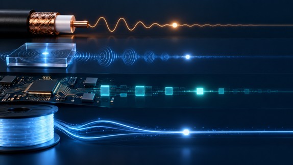
• A delay line holds back an RF signal for a precise time and is used for radar and altimeter testing, signal-path alignment, phased-array beamforming and signal processing. • The four main delay line families are coaxial cable, acoustic (SAW and BAW), digital (ADC, memory and DAC) and fiber optic. • Coax and fiber add a similar delay of roughly 4 to 5 ns per meter, but single-mode fiber loses well under 1 dB per kilometer regardless of RF frequency, while coax loss rises with length and frequency. • Emulating a radar target at 10 km needs about 66 microseconds of round-trip delay, or roughly 13.6 km of single-mode fiber. |
What is a delay line?
A delay line is a component that holds back an RF or microwave signal for a precise, known amount of time and then releases it otherwise unchanged. Delay lines are used to emulate distance in radar and altimeter testing, to align the timing of parallel signal paths, to build true-time-delay beamformers for phased arrays and to provide short-term signal memory in correlators and receivers.
In radar work the delay always represents a round trip, which makes the numbers grow quickly. A SPIE conference paper comparing microwave analog delay line technologies points out that emulating a target only 50 m away already calls for 333.33 ns of delay, because the signal has to travel out and back. For readers who want the underlying vocabulary first, a broader primer on delay lines covers the terms used throughout this comparison.
What types of delay line are available?
There are four main families of RF delay line: coaxial cable, acoustic (surface or bulk acoustic wave), digital, and fiber optic. Each creates delay in a physically different way, and that physical mechanism determines its loss, bandwidth, size and flexibility.
| Technology | How the delay is created | Main strengths | Main limitations |
| Coaxial cable | The RF signal travels through a coiled length of coax, often semi-rigid | Simple, passive, no signal conversion | Bulky at long delays; loss rises with length and frequency |
| Acoustic (SAW / BAW) | RF is converted into an acoustic wave in a piezoelectric material, which travels far slower than an electromagnetic wave | Very compact for a given delay | High insertion loss, reported above 30 dB; SAW limited to roughly 2.5 GHz |
| Digital | The signal is sampled by an ADC, held in memory and regenerated by a DAC | Delay is programmable and can be combined with synthetic Doppler or modulation | Bandwidth and spurious performance set by the converters; adds latency of its own |
| Fiber optic (ODL) | RF is modulated onto light and delayed by a chosen length of single-mode fiber | Low loss that does not change with RF frequency; delays from nanoseconds to milliseconds | Requires optical conversion, which adds noise; each delay value needs its own fiber length or a switch path |
How do coaxial delay lines compare with fiber optic delay lines?
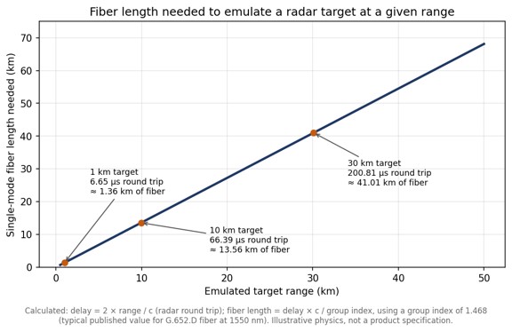
Coax and fiber produce a similar delay per meter, around 4 to 5 nanoseconds depending on the cable dielectric, but fiber achieves it with a tiny fraction of the loss. Standard G.652.D fiber has a group index close to 1.468, which works out to roughly 4.9 ns of delay per meter, or about 4.9 microseconds per kilometer.
The difference shows up in attenuation. A microsecond of delay needs roughly 200 m of either medium. Published attenuation tables put even thick 7/8-inch hardline at about 2.1 dB per 100 feet at 2.4 GHz, which means close to 14 dB of loss over 200 m, and thinner coax several times more. The same 200 m of single-mode fiber loses well under 0.1 dB of optical power. Just as important, the fiber loss is set by the optical wavelength rather than by the RF carrier riding on it, so the fiber in a fiber optic delay line contributes the same loss at 1 GHz as at 18 GHz, while a coax delay line becomes progressively lossier as frequency rises.
Longer delays make the gap decisive. The chart below shows how much fiber a radar test needs to emulate targets at different ranges. A 10 km target already requires about 13.6 km of fiber, a length no coax delay line could realistically match.
When do acoustic or digital delay lines make more sense?
Acoustic delay lines make sense when space is tight and the signal sits below a few gigahertz, and digital delay lines make sense when the delay must change continuously or the test needs synthetic signal effects. Acoustic devices exploit the fact that a mechanical wave in a piezoelectric crystal moves far more slowly than an electromagnetic wave, so a long delay fits in a small package. The cost is high insertion loss and, for surface acoustic wave parts, an upper frequency limit of around 2.5 GHz; bulk acoustic wave technology extends the achievable delay range.
A university study of wideband delay lines for automotive radar compares these approaches for a target simulator that needed an 800 MHz bandwidth and delays tunable from 1.3 ns to 1.67 microseconds, a useful example of how bandwidth and delay range together narrow the technology choice. Fully digital delay lines take a different route: an analog-to-digital converter samples the signal, memory holds it, and a digital-to-analog converter regenerates it. That flexibility is valuable, but instantaneous bandwidth, dynamic range and spurious content all depend on the converters.
What is the difference between fixed, variable and progressive delay lines?
A fixed delay line provides one delay value, while a variable delay line lets the user switch between several delays; a progressive delay line is a variable design that combines a small set of fiber spools in different combinations to produce many more delay values than it has spools. A passive optical delay line is simply a coil of fiber cut to an exact length and needs no power; in an RF system it sits between an optical transmitter and receiver.
Progressive designs typically use cascaded optical switch matrices. Four 2×2 optical switches can select 16 different delays, and eight binary-weighted spools can produce 255 distinct non-zero combinations. Variable, progressive and passive optical delay line architectures are explained in more detail, including how dispersion compensation and optical amplification are added when delays become very long.
How should an engineer choose a delay line?
Start from the application’s frequency range and maximum delay, then check loss, noise and switching requirements against each technology. The following criteria narrow the choice quickly:
- Frequency range: acoustic devices suit lower bands, while coax and fiber cover microwave frequencies and fiber holds its loss steady across them.
- Maximum delay and resolution: delays beyond a few hundred nanoseconds favor fiber; fine, continuously adjustable steps favor digital or switched designs.
- Insertion loss and noise figure: acoustic parts lose the most signal, while optical links trade a fixed conversion loss for nearly flat loss with length.
- Signal purity: phase noise and spurious content matter for radar and altimeter testing, where the delayed signal must look exactly like a real echo.
- Switching and control: test benches often need several delay values selectable from a front panel or remotely.
For signal-purity questions in optical designs, an application note on phase noise and RF amplification in ODL systems covers how amplifier placement affects the delayed signal. For catalog-level comparison of ranges and switch configurations, fiber optic delay line hardware shows how commercial units package these options into rack-mount systems.
Frequently Asked Questions
What is a delay line used for?
A delay line holds back an RF signal for a precise time, which is used to emulate target distance in radar and altimeter testing, align signal paths, steer phased-array beams and store signals briefly for processing.
How much delay does one meter of optical fiber add?
One meter of standard single-mode fiber adds roughly 4.9 nanoseconds of delay, based on a group index of about 1.468.
Why are fiber optic delay lines preferred for long delays?
Fiber optic delay lines are preferred for long delays because single-mode fiber loses well under 1 dB per kilometer and that loss does not change with the RF frequency being delayed, while coaxial cable loss grows with both length and frequency.
What is a progressive delay line?
A progressive delay line combines a small set of fiber spools through optical switches so that many delay values can be selected; eight binary-weighted spools can produce 255 different non-zero delays.
Buildings, tunnels, and parking structures block GPS satellite signals from reaching the devices that depend on them for precise timing. Distributing a single rooftop GPS signal to many indoor locations without losing accuracy is a common, and often underestimated, engineering problem. This piece walks through how GPS over fiber distribution solves it, in plain question-and-answer form.
Why can’t you just run coax to every timing device?
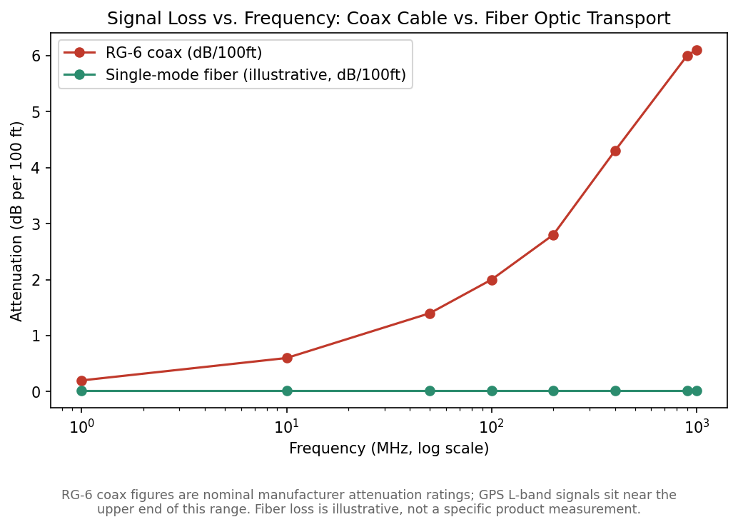
Coaxial cable loses signal strength as it gets longer, and that loss gets worse at higher frequencies. GPS signals sit up near 1.5 GHz, a range where coax attenuation climbs quickly. Once a cable run stretches beyond roughly a hundred feet, the accumulated loss can degrade the signal below what a receiver needs to lock onto it reliably.
Nominal coax attenuation rises steeply with frequency, while fiber optic loss stays comparatively flat and low (illustrative, not a specific product measurement).
How does the fiber-based alternative work?
A rooftop GPS antenna feeds a transmitter module that converts the incoming satellite signal onto an optical carrier. That optical signal travels over low-loss fiber, and can be split to reach many destinations at once using standard optical splitters, before a fiber optic transmitter and receiver pair converts each branch back to an RF GPS signal at its endpoint. Because a single donor antenna can feed dozens of splits, one rooftop receiver can serve timing devices scattered across an entire facility.
What actually needs this kind of precise timing?
Data centers rely on GPS timing to keep distributed systems synchronized. Financial networks use it to timestamp transactions consistently across locations. Highway tunnels sometimes need GPS re-radiated inside for emergency vehicle navigation. In each case the requirement is the same: get an accurate, undistorted GPS signal to a location the satellite signal itself can’t reach directly.
How precise does GPS timing actually get?
According to the U.S. government’s official GPS information site, GPS time transfer is commonly used to synchronize clocks and networks to Coordinated Universal Time, with a typical accuracy relative to the U.S. Naval Observatory’s time standard of 30 nanoseconds or better, 95 percent of the time, when using a dedicated time-transfer receiver. See GPS.gov’s overview of GPS timing applications for more detail on how that precision is used across industries.
Frequently Asked Questions
Why does GPS signal distribution need fiber instead of just more coax?
Coax loss increases sharply at GPS frequencies, so runs longer than about a hundred feet start to degrade signal quality. Fiber optic loss stays low over much longer distances.
Can one GPS antenna really serve an entire building?
Yes. Once the signal is converted to an optical carrier, it can be split many times using standard optical splitters, letting a single rooftop antenna feed numerous indoor endpoints.
What industries rely most on distributed GPS timing?
Data centers, financial networks, and telecommunications infrastructure are common users, since all depend on precise, synchronized time across multiple locations.
Among the most widely used IC packages in modern electronics, QFN packages have earned their place in product designs ranging from Bluetooth chips to automotive radar modules. Compact, thermally efficient, and electrically clean, QFN (Quad Flat No-Lead) packages offer a compelling combination of performance and manufacturability. But not all QFN packages are equal — and the differences between standard, organic, and panel-level variants can significantly affect both product performance and production economics.
This article breaks down the key QFN package types, explores their respective advantages, and explains how advances in panel-level packaging are reshaping the economics of high-volume production.
What Is a QFN Package?
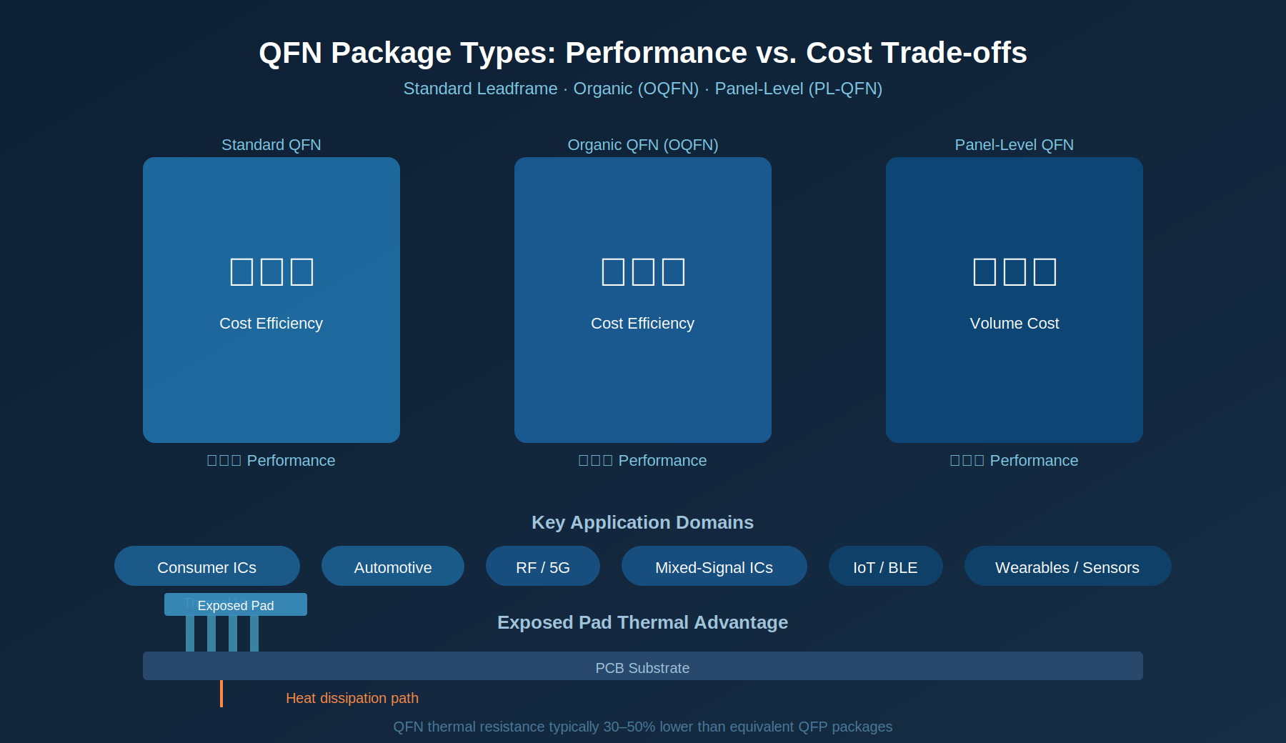
QFN stands for Quad Flat No-Lead — a surface-mount package format where leads are located on the underside of the package rather than extending outward. A large exposed pad on the package bottom provides a direct thermal path to the PCB, making QFN one of the most thermally efficient small-form-factor package types available.
The absence of external leads reduces parasitic inductance and capacitance compared to gull-wing leaded packages, improving high-frequency performance. This combination of thermal and electrical benefits has made QFN the package of choice across consumer electronics, wireless communications, industrial sensors, and automotive control units.
QFN Package Types: A Comparison
While the QFN concept is consistent, several variants have emerged to serve different manufacturing processes and performance requirements:
| Package Variant | Process Basis | Key Advantage | Typical Use |
| Standard QFN | Leadframe + molding | Low cost, mature supply chain | Consumer ICs, PMIC |
| Organic QFN (OQFN) | Organic substrate | Finer pitch, better signal integrity | RF, telecom, mixed-signal |
| Panel-Level QFN (PL-QFN) | Panel-level packaging | Ultra-low cost at volume | IoT, wearables, automotive |
| Dual-Row QFN | Leadframe | Higher I/O density | Connectivity ICs |
| Thermally Enhanced QFN | Leadframe + thermal slug | Superior heat dissipation | Power semiconductors |
Organic QFN: The High-Performance Alternative
Traditional QFN packages use a metal leadframe as the substrate — a cost-effective approach that suits high-volume commodity ICs. Organic QFN replaces the leadframe with an organic laminate substrate, enabling finer pitch routing, better impedance control, and improved electrical performance for RF and mixed-signal applications.
For RF front-end modules, millimeter-wave components, and precision analog ICs, organic QFN delivers performance characteristics that leadframe-based packages cannot match. The substrate enables multi-layer routing, embedded passive integration, and support for tighter pad pitches demanded by advanced silicon nodes.
PCB Technologies’ iNPACK division has developed deep capabilities in organic QFN manufacturing, offering DFM consultation, rapid prototyping, and scalable production. Their approach ensures that performance-optimized designs translate successfully from simulation to silicon.
Panel-Level Packaging: The Cost Revolution
Wafer-level packaging has long been the benchmark for cost-efficient IC packaging in high-volume production — but it is constrained by wafer diameter. Panel-level packaging applies the same lithographic and encapsulation processes to rectangular panels many times larger than a 300mm wafer, dramatically increasing throughput per equipment cycle.
For QFN-type packages produced at scale, panel-level processing can reduce per-unit cost by 30–50% compared to wafer-level equivalents, depending on die size and panel utilization. This cost structure is transforming the economics of IoT components, wireless modules, and automotive sensor ICs — categories where per-unit price pressure is intense.
Thermal Management in QFN Designs
One of the most critical design decisions when using QFN packages is thermal management at the board level. The exposed thermal pad requires careful PCB design to maximize heat transfer:
- Thermal via arrays beneath the exposed pad are strongly recommended for high-power devices
- Pad size should follow IPC-7351 land pattern guidelines for the specific package
- Solder paste aperture design affects both electrical connection and thermal conductivity
- Adjacent ground planes and copper pours help spread heat away from the die
Poor thermal design with QFN packages can negate their inherent thermal advantage, resulting in premature failure or derating. PCB Technologies provides DFM review as part of their packaging engagement, catching thermal design issues before they reach prototype stage.
QFN vs. QFP: When Each Makes Sense
The most common comparison made against QFN is QFP (Quad Flat Package) — the leaded alternative. Each format has its place:
- QFN: Better for high-frequency applications, tighter board area budgets, and superior thermal performance; requires precision solder printing
- QFP: Easier to inspect visually and rework, more forgiving of PCB assembly tolerances; larger footprint
For new designs targeting advanced nodes and compact form factors, QFN consistently wins the performance-per-area tradeoff. The manufacturing challenge of QFN — particularly solder void management under the thermal pad — is well-understood and manageable with proper process controls.
PCB Technologies’ QFN Capability
PCB Technologies offers end-to-end QFN packaging services through their iNPACK platform, spanning design consultation, substrate development, packaging, and test. Their organic QFN capabilities support pitches not achievable with standard leadframe-based processes, making them a strong partner for next-generation wireless, automotive, and medical IC designs.
With established supply chains for organic substrate materials and a track record across demanding qualification standards, PCB Technologies bridges the gap between the cost efficiency demanded by volume production and the performance requirements of advanced applications.
Conclusion
QFN packages continue to evolve — from standard leadframe variants to organic and panel-level formats that unlock new performance and cost tiers. As silicon advances drive smaller die sizes and higher I/O densities, the packaging layer becomes increasingly critical. Selecting the right QFN variant and working with an experienced packaging partner ensures that board-level performance matches the potential of the silicon within.

The AI Isn’t Wrong About Your Company. Your Sources Are | Interview with Aia Laser

Should B2B Brands Optimize for Specific AI Engines? How ChatGPT, Google, Perplexity, and Claude Compare

What Is a Blow Molded Case? Process, Materials and Trade-offs Explained

-

 Business Solutions2 years ago
Live Video Broadcasting with Bonded Transmission Technology
-

 Business Solutions2 years ago
The Future of Healthcare SMS and RCS Messaging
-

 Business Solutions2 years ago
2-Way Texting Solutions from Company Message Services
-

 Business Solutions2 years ago
Communication with Analog to Fiber Converters & RF Link Budgets
-

 DSRC Communication2 years ago
The Crossroads of Connectivity: DSRC vs. C-V2X Technologies in Automotive Communication
-

 Business Solutions2 years ago
Wholesale SMS Platforms with OTP Services
-

 Business Solutions2 years ago
Choosing the Right B2B Digital Marketing Agency: A Guide
-

 3D Technology2 years ago
How Multispectral Cameras Advance Book Scanning